Introduction
Introduction.RmdbiomeViz
biomeViz is part of the RIVM-ToolBox project aimed at
providing standard set of tools that interact with open tools for a wide
array of data analytics, including microbiomics. The RIVM-ToolBox is a
set of individual R tools focused towards different
goals/functionalities.
biomeUtils: Data handling
Outputs for standard data generating pipelines/workflows.biomeStats: Data analytics
Common data analytics including basic statistics.biomeViz: Data visualization
Data visualization of different data types.
library(biomeViz)
#> Loading required package: phyloseq
#> Loading required package: biomeUtils
#> Loading required package: microbiome
#> Loading required package: ggplot2
#>
#> microbiome R package (microbiome.github.com)
#>
#>
#>
#>  Copyright (C) 2011-2022 Leo Lahti,
#>     Sudarshan Shetty et al. <microbiome.github.io>
#>
#> Attaching package: 'microbiome'
#> The following object is masked from 'package:ggplot2':
#>
#>     alpha
#> The following object is masked from 'package:base':
#>
#>     transform
Categorical and numeric plot
Visualize one categorical column and one numeric column in
sample_data.
library(biomeUtils)
library(biomeViz)
library(dplyr)
library(microbiome)
library(ggplot2)
library(gghalves)
library(patchwork)

ps <- FuentesIliGutData
# calculate Shannon diversity using microbiome::diversity and add it to
# the sample_data in phyloseq using biomeUtils::mutateSampleData()
ps <- mutateSampleData(ps,
                       Shannon = microbiome::diversity(ps, "shannon")[,1])
plotByGroup(ps,
            x.factor="ILI",
            y.numeric = "Shannon") +
  gghalves::geom_half_point(
    ggplot2::aes_string(fill="ILI"),
    side = "l",
    range_scale = .4,
    alpha = 0.25,
    shape = 21) +
  scale_fill_manual(values = c("#3d6721", "#a86826", "#006c89"), guide = "none")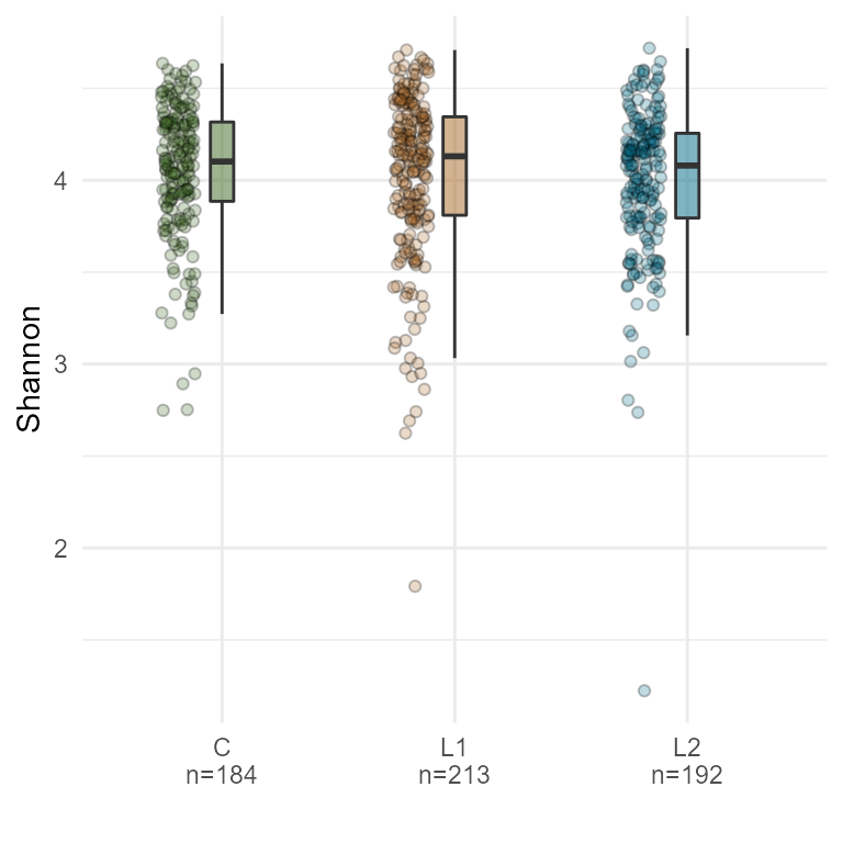
Scatter plot
library(biomeUtils)
library(biomeViz)
library(dplyr)
library(microbiome)
library(ggplot2)
plotScatterViz(ps, x_numeric = "Shannon", y_numeric = "BMI",
               color_var = "ILI") +
  scale_fill_manual(values=c("steelblue", "brown3", "grey70"))+
  scale_fill_manual(values=c("steelblue", "brown3", "grey70"))
#> Registered S3 method overwritten by 'ggside':
#>   method from
#>   +.gg   ggplot2
#> Scale for 'fill' is already present. Adding another scale for 'fill', which
#> will replace the existing scale.
#> Warning: Removed 1 rows containing non-finite values (stat_density).
#> Warning: Removed 1 rows containing missing values (geom_point).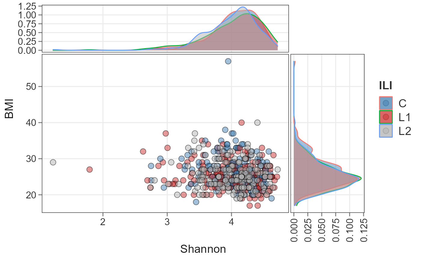
Theme showcase
p.base <- plotByGroup(ps,
                      x.factor="ILI",
                      y.numeric = "Shannon") +
  gghalves::geom_half_point(
    ggplot2::aes_string(fill="ILI"),
    side = "l",
    range_scale = .4,
    alpha = 0.25,
    shape = 21) +
  labs(subtitle = "base plot") +
  theme_bw() +
  scale_fill_biomeViz(palette = "viz3")


p.bw <- plotByGroup(ps,
                    x.factor="ILI",
                    y.numeric = "Shannon") +
  gghalves::geom_half_point(
    ggplot2::aes_string(fill="ILI"),
    side = "l",
    range_scale = .4,
    alpha = 0.25,
    shape = 21) +
  scale_fill_biomeViz(palette = "viz3") +
  labs(subtitle = "biomeViz bw") +
  theme_biomViz_bw()

p.min <- plotByGroup(ps,
                    x.factor="ILI",
                    y.numeric = "Shannon") +
  gghalves::geom_half_point(
    ggplot2::aes_string(fill="ILI"),
    side = "l",
    range_scale = .4,
    alpha = 0.25,
    shape = 21) +
  scale_fill_biomeViz(palette = "viz3") +
  labs(subtitle = "biomeViz minimal") +
  theme_biomViz_minimal()

p.gen <- plotByGroup(ps,
                    x.factor="ILI",
                    y.numeric = "Shannon") +
  gghalves::geom_half_point(
    ggplot2::aes_string(fill="ILI"),
    side = "l",
    range_scale = .4,
    alpha = 0.25,
    shape = 21) +
  scale_fill_biomeViz(palette = "viz3") +
  labs(subtitle = "biomeViz general") +
  theme_biomViz()

((p.base | p.bw )  / ( p.min  | p.gen ) ) + plot_layout(guides = "collect")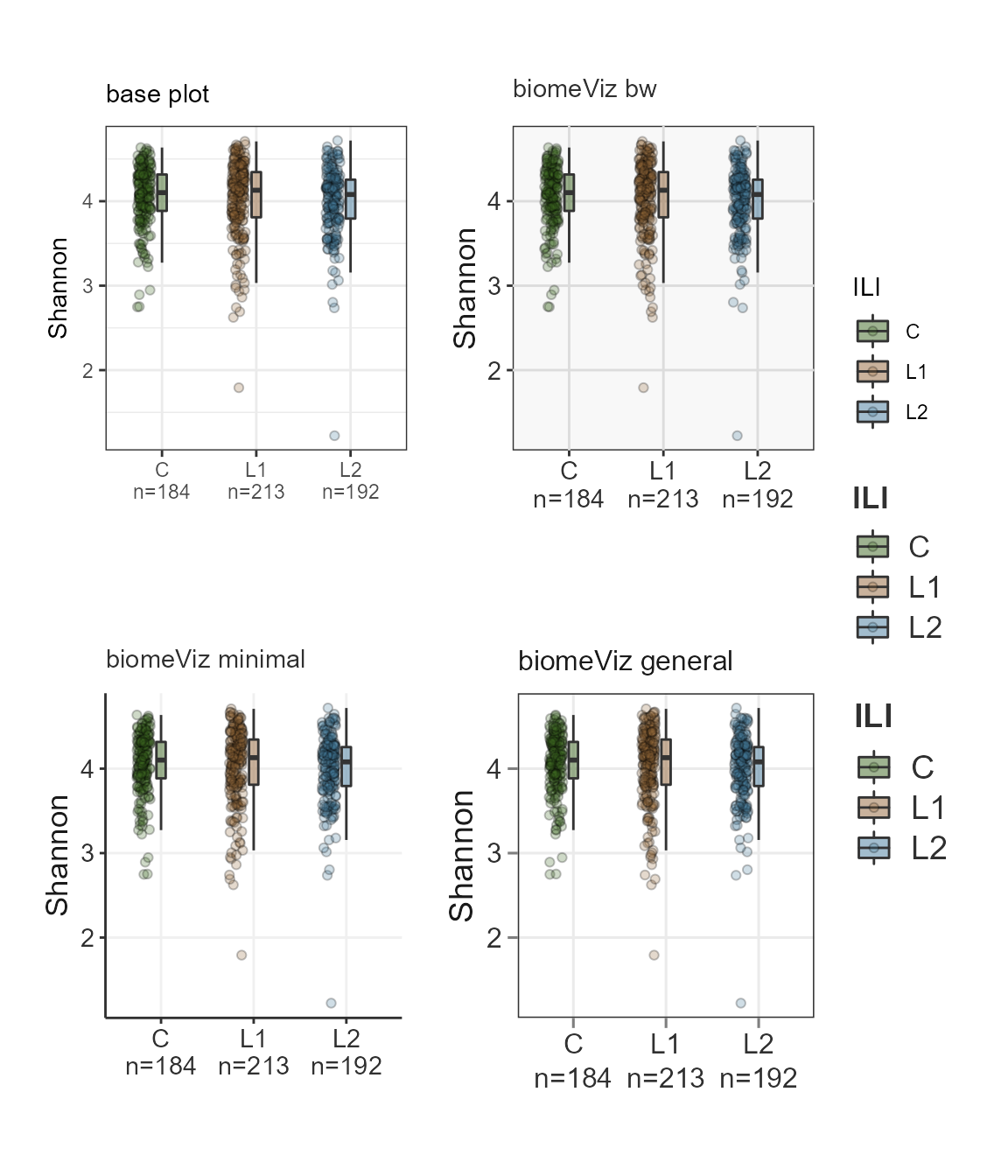
Top features
Plot the features with the highest abundance in all samples.
library(biomeUtils)
library(biomeViz)
plotTopAbundant(SprockettTHData,
                taxa_level = "Family",
                top=10L,
                aes(color=Phylum)) +
  theme_biomViz_minimal() +
  scale_colour_biomeViz_summer()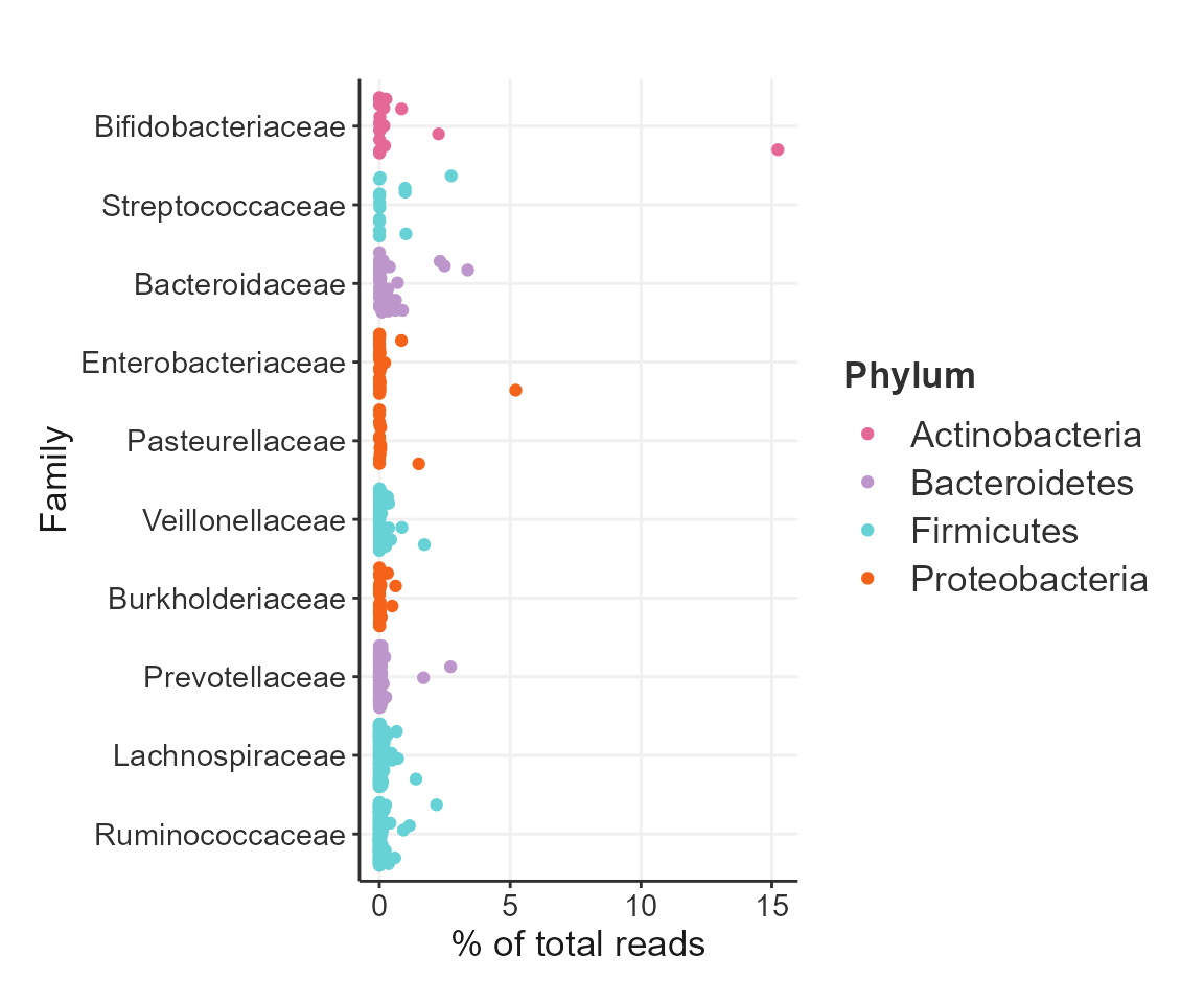
Heatmap
library(biomeUtils)
library(biomeViz)
library(microbiome)
library(dplyr)
library(tidyHeatmap)

#  Transform to relative abundance
ps <- FuentesIliGutData %>%
  microbiome::transform("compositional")

# Select taxa to plot. This avoid overcrowding
select_taxa <- findTopTaxa(ps, top= 10, method="mean")

p <- plotTidyHeatmap(ps, select_taxa = select_taxa,
                     group_samples_by = "ILI",
                     add_taxa_label = FALSE,
                     cluster_rows = FALSE,
                     .scale = "none", # no scaling only relative abundance
                     transform = NULL,
                     palette_grouping = list(biomeViz_palettes$viz3)) %>%
  add_line(age)
p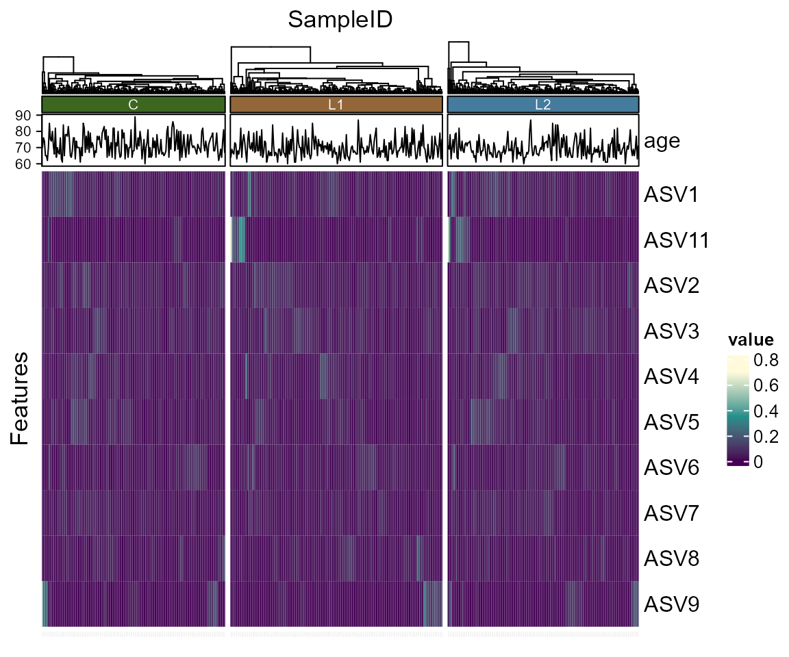
Raincloud
Rain clouds are effective to visualize data. Read more about their utility here Allen M, Poggiali D, Whitaker K et al. Raincloud plots: a multi-platform tool for robust data visualization [version 2; peer review: 2 approved]. Wellcome Open Res 2021, 4:63 link
library(biomeUtils)
library(biomeViz)
library(microbiome)
library(ggplot2)
library(dplyr)

ps <- FuentesIliGutData %>%
  microbiome::aggregate_taxa("Genus") %>%
  microbiome::transform("compositional")

plotTaxaRaincloud(ps,
                  taxa ="Bacteroides",
                  group_samples_by = "ILI",
                  opacity = 0.25,
                  shape_point = 21) + # combine with ggplot2 for improvements
  labs(y = "Relative abundance",
       x = "",
       subtitle = expression(paste("Raincloud plot showing the distribution of ",italic("Bacteroides")))) +
  theme_biomViz()+
  scale_fill_manual(values = c("#3d6721", "#a86826", "#006c89"), guide = "none") +
  scale_color_manual(values = c("#3d6721", "#a86826", "#006c89"), guide = "none") +
  theme(plot.subtitle = element_text(margin = margin(t = 5, b = 10)),
plot.margin = margin(10, 25, 10, 25)) 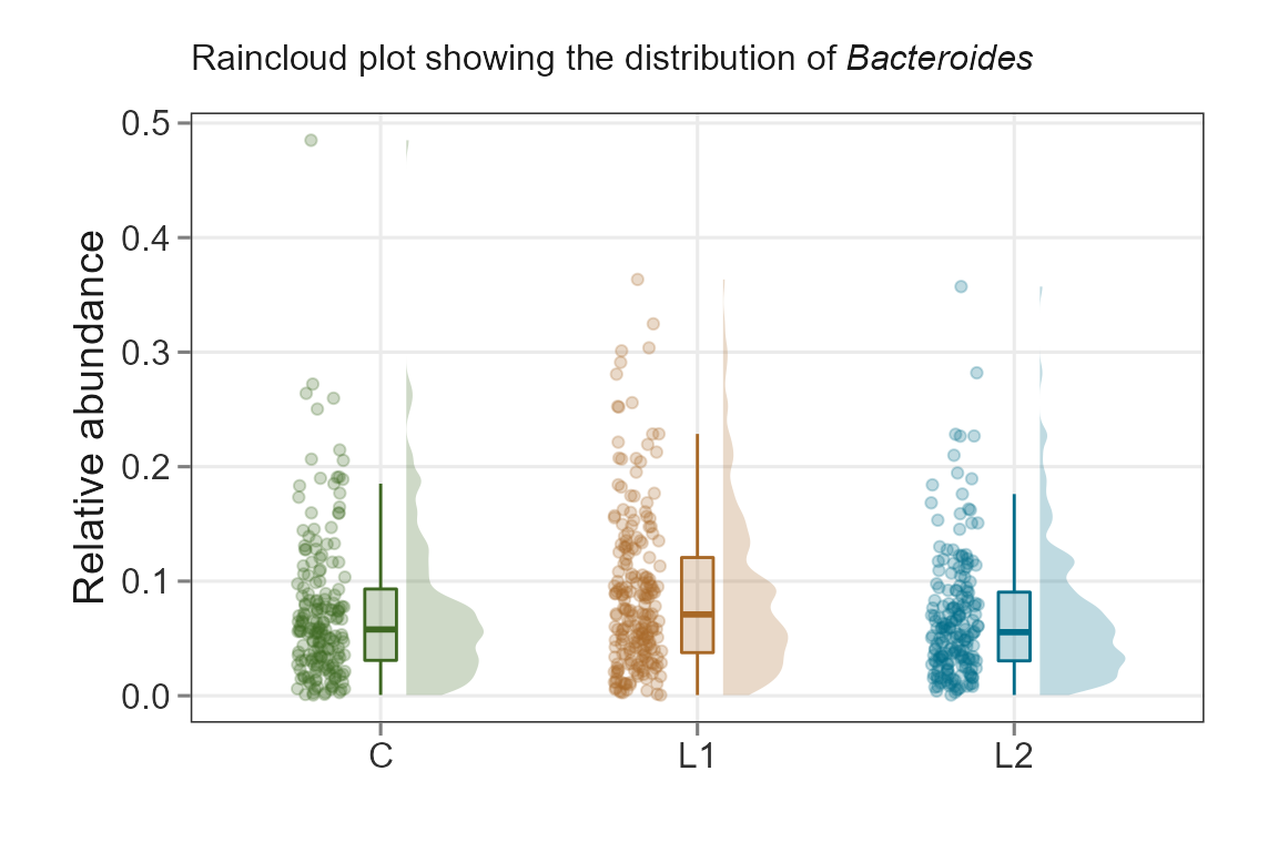
Plot CLR abundance of multiple taxa.
ps <- FuentesIliGutData %>%
  microbiome::aggregate_taxa("Genus") %>%
  microbiome::transform("clr")

taxa.to.plot <- c("Bacteroides","Blautia","Roseburia","Faecalibacterium")

plotTaxaRaincloud(ps,
                  taxa = taxa.to.plot,
                  group_samples_by = "ILI",
                  opacity = 0.25,
                  shape_point = 21) + # combine with ggplot2 for improvements
  labs(y = "CLR Abundance",
       x = "") +
  theme_biomViz_bw() +
  theme(strip.text.x = element_text(face = "italic")) +
  scale_fill_manual(values = c("#3d6721", "#a86826", "#006c89"), guide = "none") +
scale_color_manual(values = c("#3d6721", "#a86826", "#006c89"), guide = "none") 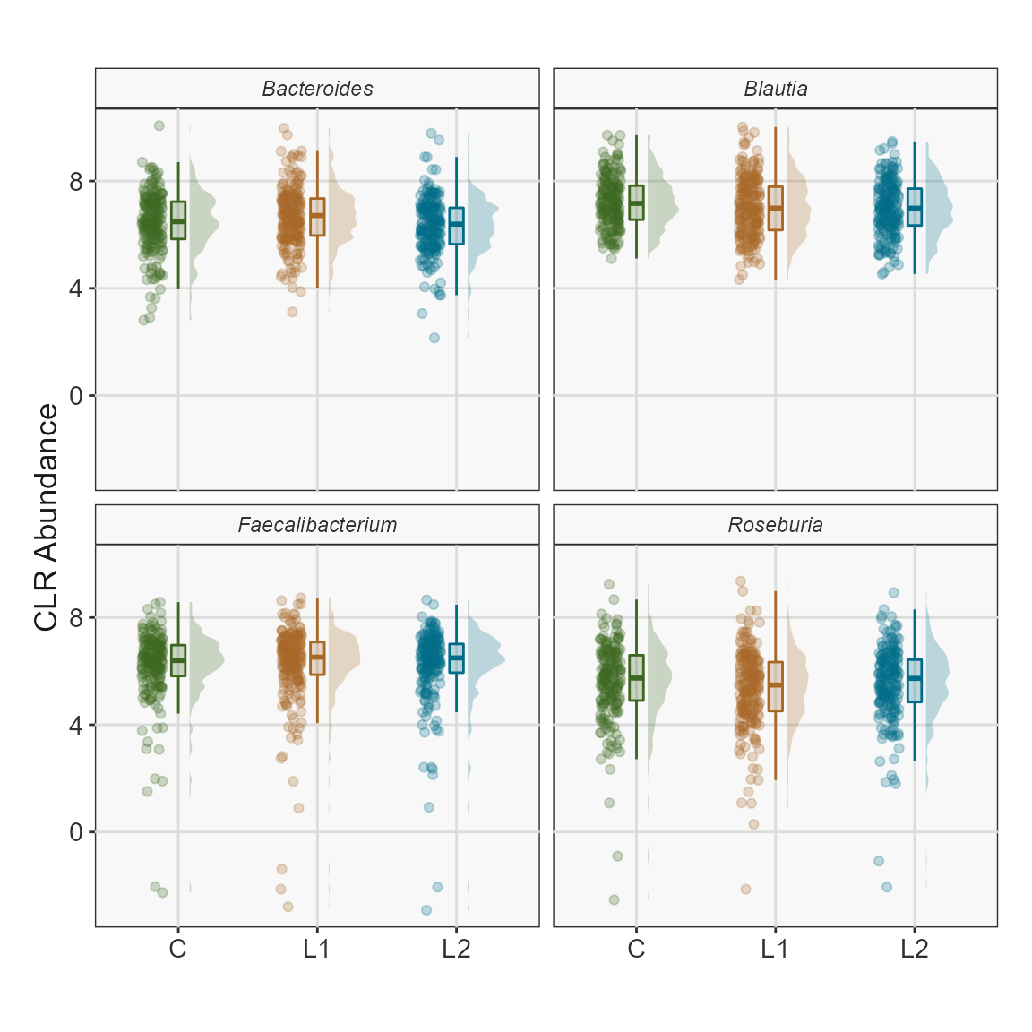
PCoA plot
A Principal Coordinates Analysis for phyloseq object. To
visualize similarities/dissimilarities between samples in 2D ordination.
This function extends the phyloseq ordination plots to
include taxa that correlate with chosen axis and plots them along with a
side boxplot for comparing inter-sample variation within groups.
library(biomeUtils)
library(dplyr)
library(ggside)
ps <- FuentesIliGutData %>%
  microbiome::transform("compositional") %>%
  mutateTaxaTable(FeatureID = taxa_names(FuentesIliGutData))
plotPCoA(x =ps,
         group_var = "ILI",
         ord_method = "PCoA",
         dist_method = "bray",
         seed = 1253,
         cor_method = "spearman",
         verbose = TRUE,
         padj_cutoff = 0.05,
         padj_method = "fdr",
         arrows = TRUE,
         label_col = "grey30",
         plot_centroids = TRUE,
         add_side_box = TRUE,
         axis_plot = c(1:2),
         point_shape = 21,  # point_shape
         point_alpha = 0.5) +
  theme_biomViz_minimal() +
  scale_color_manual(values = c("#3d6721", "#a86826", "#006c89")) +
  scale_fill_manual(values = c("#3d6721", "#a86826", "#006c89"))
#> Random number for permutation analysis ...
#> 1253
#> 'adonis' will be deprecated: use 'adonis2' instead
#> Warning in .check_taxa_axis(axis.a.tax, axis.b.tax): Second of the choosen axis
#> in `axis_plot` has no taxa satisfying criteria to plot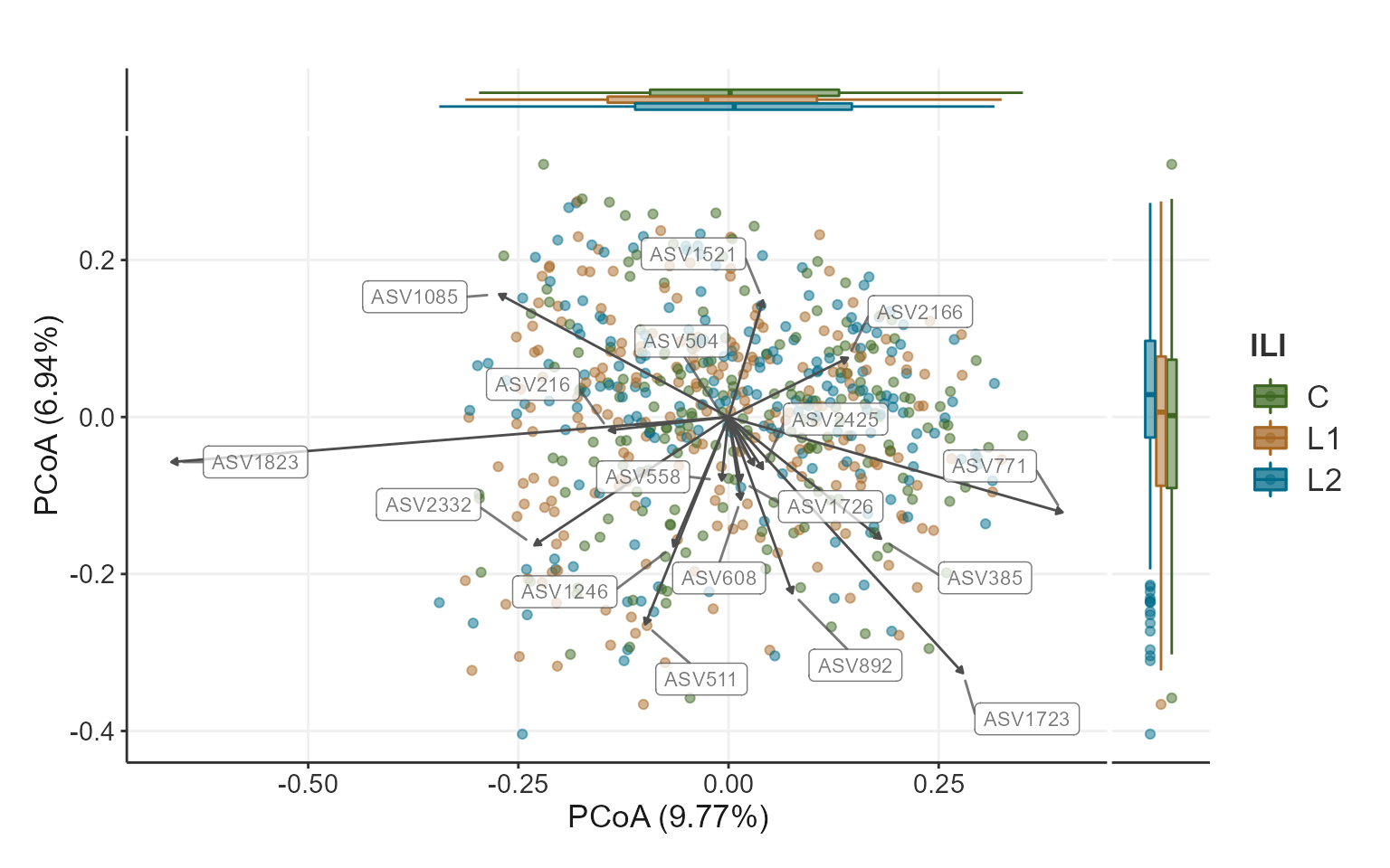
sessionInfo()
#> R version 4.2.1 (2022-06-23 ucrt)
#> Platform: x86_64-w64-mingw32/x64 (64-bit)
#> Running under: Windows 10 x64 (build 19044)
#>
#> Matrix products: default
#>
#> locale:
#> [1] LC_COLLATE=English_United States.utf8
#> [2] LC_CTYPE=English_United States.utf8
#> [3] LC_MONETARY=English_United States.utf8
#> [4] LC_NUMERIC=C
#> [5] LC_TIME=English_United States.utf8
#>
#> attached base packages:
#> [1] stats     graphics  grDevices utils     datasets  methods   base
#>
#> other attached packages:
#>  [1] ggside_0.2.0      tidyHeatmap_1.8.1 patchwork_1.1.1   gghalves_0.1.3
#>  [5] dplyr_1.0.9       biomeViz_0.0.06   biomeUtils_0.018  microbiome_1.18.0
#>  [9] ggplot2_3.3.6     phyloseq_1.40.0
#>
#> loaded via a namespace (and not attached):
#>   [1] Rtsne_0.16             colorspace_2.0-3       rjson_0.2.21
#>   [4] ellipsis_0.3.2         rprojroot_2.0.3        circlize_0.4.15
#>   [7] XVector_0.36.0         GlobalOptions_0.1.2    fs_1.5.2
#>  [10] clue_0.3-61            rstudioapi_0.13        farver_2.1.0
#>  [13] ggrepel_0.9.1          bit64_4.0.5            fansi_1.0.3
#>  [16] codetools_0.2-18       splines_4.2.1          doParallel_1.0.17
#>  [19] cachem_1.0.6           knitr_1.39             ade4_1.7-19
#>  [22] jsonlite_1.8.0         cluster_2.1.3          png_0.1-7
#>  [25] ggdist_3.1.1           compiler_4.2.1         assertthat_0.2.1
#>  [28] Matrix_1.4-1           fastmap_1.1.0          cli_3.3.0
#>  [31] htmltools_0.5.2        tools_4.2.1            igraph_1.3.1
#>  [34] gtable_0.3.0           glue_1.6.2             GenomeInfoDbData_1.2.8
#>  [37] reshape2_1.4.4         fastmatch_1.1-3        Rcpp_1.0.8.3
#>  [40] Biobase_2.56.0         jquerylib_0.1.4        pkgdown_2.0.5
#>  [43] vctrs_0.4.1            Biostrings_2.64.0      rhdf5filters_1.8.0
#>  [46] multtest_2.52.0        ape_5.6-2              nlme_3.1-157
#>  [49] DECIPHER_2.24.0        iterators_1.0.14       xfun_0.31
#>  [52] stringr_1.4.0          lifecycle_1.0.1        phangorn_2.8.1
#>  [55] dendextend_1.15.2      zlibbioc_1.42.0        MASS_7.3-57
#>  [58] scales_1.2.0           ragg_1.2.2             parallel_4.2.1
#>  [61] biomformat_1.24.0      rhdf5_2.40.0           RColorBrewer_1.1-3
#>  [64] ComplexHeatmap_2.12.0  yaml_2.3.5             gridExtra_2.3
#>  [67] memoise_2.0.1          sass_0.4.1             stringi_1.7.6
#>  [70] RSQLite_2.2.14         highr_0.9              S4Vectors_0.34.0
#>  [73] desc_1.4.1             foreach_1.5.2          permute_0.9-7
#>  [76] BiocGenerics_0.42.0    shape_1.4.6            GenomeInfoDb_1.32.2
#>  [79] rlang_1.0.2            pkgconfig_2.0.3        systemfonts_1.0.4
#>  [82] bitops_1.0-7           matrixStats_0.62.0     distributional_0.3.0
#>  [85] evaluate_0.15          lattice_0.20-45        purrr_0.3.4
#>  [88] Rhdf5lib_1.18.2        labeling_0.4.2         bit_4.0.4
#>  [91] tidyselect_1.1.2       plyr_1.8.7             magrittr_2.0.3
#>  [94] R6_2.5.1               IRanges_2.30.0         generics_0.1.2
#>  [97] picante_1.8.2          DBI_1.1.3              pillar_1.7.0
#> [100] withr_2.5.0            mgcv_1.8-40            survival_3.3-1
#> [103] RCurl_1.98-1.6         tibble_3.1.7           crayon_1.5.1
#> [106] utf8_1.2.2             rmarkdown_2.14         viridis_0.6.2
#> [109] GetoptLong_1.0.5       grid_4.2.1             data.table_1.14.2
#> [112] blob_1.2.3             vegan_2.6-2            digest_0.6.29
#> [115] tidyr_1.2.0            textshaping_0.3.6      stats4_4.2.1
#> [118] munsell_0.5.0          viridisLite_0.4.0      bslib_0.3.1
#> [121] quadprog_1.5-8