biomeUtils
biomeUtils is part of the RIVM-ToolBox project aimed at
providing standard set of tools that interact with open tools for a wide
array of data analytics, including microbiomics. The RIVM-ToolBox is a
set of individual R tools focused towards different
goals/functionalities.
biomeUtils: Data handling
Outputs for standard data generating pipelines/workflows.biomeStats: Data analytics
Common data analytics including basic statistics.biomeViz: Data visualization
Data visualization of different data types.
Setup
Install
devtools::install_github("RIVM-IIV-Microbiome/biomeUtils")Load pkg
library(biomeUtils)
#> Loading required package: phyloseq
#> Loading required package: microbiome
#> Loading required package: ggplot2
#>
#> microbiome R package (microbiome.github.com)
#>
#>
#>
#>  Copyright (C) 2011-2022 Leo Lahti,
#>     Sudarshan Shetty et al. <microbiome.github.io>
#>
#> Attaching package: 'microbiome'
#> The following object is masked from 'package:ggplot2':
#>
#>     alpha
#> The following object is masked from 'package:base':
#>
#>     transform
Data handling
Data
data("FuentesIliGutData")
FuentesIliGutData
#> phyloseq-class experiment-level object
#> otu_table()   OTU Table:         [ 905 taxa and 589 samples ]
#> sample_data() Sample Data:       [ 589 samples by 61 sample variables ]
#> tax_table()   Taxonomy Table:    [ 905 taxa by 7 taxonomic ranks ]
#> phy_tree()    Phylogenetic Tree: [ 905 tips and 904 internal nodes ]
Get tibbles
data("FuentesIliGutData")
# get otu table in tibble format
otu_tib <- getAbundanceTibble(FuentesIliGutData,
                              select_rows = c("ASV302", "ASV82", "ASV410", "ASV2332"),
                              select_cols = c("sample_1", "sample_5", "sample_6"),
                              column_id = "FeatureID")

# get taxa table in tibble format
tax_tib <- getTaxaTibble(FuentesIliGutData,
                         select_rows = c("ASV302", "ASV82", "ASV410", "ASV2332"),
                         select_cols = c("Phylum", "Genus"),
                         column_id = "FeatureID")

# get sample data in tibble format
meta_tib <- getSampleTibble(FuentesIliGutData,
                            select_rows = c("sample_1", "sample_5", "sample_6"),
                            select_cols = c("participant_id", "ILI", "age"),
                            column_id = "FeatureID")
Subset/Filter phyloseq
# Filter by phyloseq like subset_*
ps.filtered.samples  <- filterSampleData(FuentesIliGutData,
                                         ILI == "C" & BMI < 26)
ps.filtered.samples
#> phyloseq-class experiment-level object
#> otu_table()   OTU Table:         [ 901 taxa and 91 samples ]
#> sample_data() Sample Data:       [ 91 samples by 61 sample variables ]
#> tax_table()   Taxonomy Table:    [ 901 taxa by 7 taxonomic ranks ]
#> phy_tree()    Phylogenetic Tree: [ 901 tips and 900 internal nodes ]

ps.filtered.taxa  <- filterTaxaData(FuentesIliGutData,
                                    Phylum=="Firmicutes")

ps.filtered.taxa
#> phyloseq-class experiment-level object
#> otu_table()   OTU Table:         [ 758 taxa and 589 samples ]
#> sample_data() Sample Data:       [ 589 samples by 61 sample variables ]
#> tax_table()   Taxonomy Table:    [ 758 taxa by 7 taxonomic ranks ]
#> phy_tree()    Phylogenetic Tree: [ 758 tips and 757 internal nodes ]

# Filter by names like prune_*
sams.select <- sample_names(FuentesIliGutData)[1:10]
ps.filter.by.sam.names <- filterSampleByNames(FuentesIliGutData,
                                               ids = sams.select,
                                               keep = TRUE)

tax.select <- taxa_names(FuentesIliGutData)[1:10]
ps.filter.by.tax.names <- filterTaxaByNames(FuentesIliGutData,
                                           ids = tax.select,
                                           keep = TRUE)
Check for polyphyly
Check for polyphyletic taxa in tax_table. Useful to
check this before aggregating at any level. Here, for
e.g. Eubacterium is is in both Lachnospiraceae and
EUbacteriaceae family.
library(biomeUtils)
library(dplyr)
#>
#> Attaching package: 'dplyr'
#> The following objects are masked from 'package:stats':
#>
#> filter, lag
#> The following objects are masked from 'package:base':
#>
#> intersect, setdiff, setequal, union
data("FuentesIliGutData")
polydf <- checkPolyphyletic(FuentesIliGutData,
taxa_level = "Genus",
return_df = TRUE)
polydf
#> # A tibble: 6 × 7
#> # Groups: Genus [3]
#> Domain Phylum Class Order Family Genus nfeat…¹
#> <chr> <chr> <chr> <chr> <chr> <chr> <int>
#> 1 Bacteria Firmicutes Clostridia Clostridiales Lachnospiraceae Eubacter… 2
#> 2 Bacteria Firmicutes Clostridia Clostridiales Lachnospiraceae Clostrid… 2
#> 3 Bacteria Firmicutes Clostridia Clostridiales Lachnospiraceae Ruminoco… 2
#> 4 Bacteria Firmicutes Clostridia Clostridiales Ruminococcaceae Ruminoco… 2
#> 5 Bacteria Firmicutes Clostridia Clostridiales Eubacteriaceae Eubacter… 2
#> 6 Bacteria Firmicutes Clostridia Clostridiales Ruminococcaceae Clostrid… 2
#> # … with abbreviated variable name ¹nfeaturesCompare phyloseqs
library(biomeUtils)
data("FuentesIliGutData")
ps1 <- filterSampleData(FuentesIliGutData, ILI == "C")

ps2 <- filterSampleData(FuentesIliGutData, ILI == "L1")

ps3 <- filterSampleData(FuentesIliGutData, ILI == "L2")


ps.list <- c("C" = ps1, "L1" = ps2, "L2" = ps3)

comparePhyloseq(ps.list)
#>   input ntaxa nsample min.reads max.reads total.read average.reads singletons
#> 1     C   901     184     10975    143946    7658743      41623.60          0
#> 2    L1   902     213     12715    140779    8568244      40226.50          0
#> 3    L2   896     192     24868    194135   15127300      78788.02          0
#>    sparsity
#> 1 0.6717355
#> 2 0.6678794
#> 3 0.6372652
Calculations
Phylogenetic diversity
library(biomeUtils)
data("FuentesIliGutData")
# reduce size for example
ps1 <- filterSampleData(FuentesIliGutData, ILI == "C")

meta_tib <- calculatePD(ps1, justDF=TRUE)
# check
meta_tib[c(1,2,3),c("PD", "SR")]
Prevalence
data("FuentesIliGutData")
prev_tib <- getPrevalence(FuentesIliGutData,
                          return_rank= c("Family", "Genus"),
                          return_taxa = c("ASV4", "ASV17" , "ASV85", "ASV83"),
                          sort=TRUE)
head(prev_tib)
#>    Taxa prevalence           Family         Genus
#> 1  ASV4  0.9881154  Lachnospiraceae       Blautia
#> 2 ASV17  0.9847199 Streptococcaceae Streptococcus
#> 3 ASV85  0.7758913  Lachnospiraceae     Roseburia
#> 4 ASV83  0.7045840   Bacteroidaceae   Bacteroides
Microbiota Uniqueness
Extracts the minimum value from a matrix for each individual. This is the dissimilarity of an individual from their nearest neighbor. Here, the option of using a one or more reference samples is provided. see the man page. The original article (cite when using this) did all versus all samples dissimilarities. Wilmanski T, et al., (2021) Gut microbiome pattern reflects healthy ageing and predicts survival in humans. Nature metabolism
library(biomeUtils)
data("FuentesIliGutData")
ps <- getProportions(FuentesIliGutData)
dist.mat <- phyloseq::distance(ps, "bray")
muniq <- uniqueness(ps,
                    dist_mat=dist.mat,
                    reference_samples = NULL)
#head(muniq)

ggplot(muniq,aes(age,uniqueness)) +
  geom_point(alpha=0.5) +
  geom_smooth(method = "lm") +
  theme_bw()
#> `geom_smooth()` using formula 'y ~ x'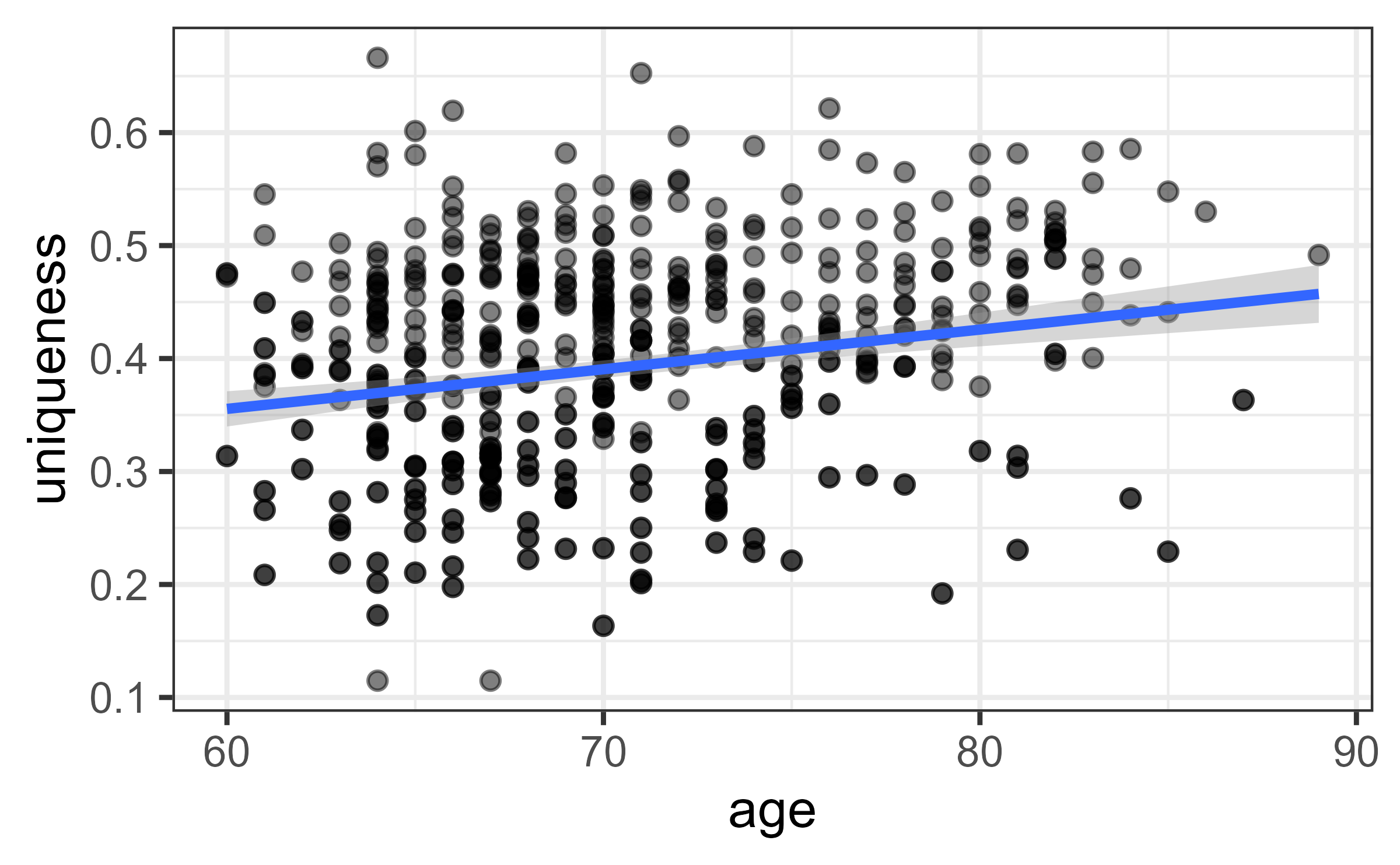
Fold Difference
library(biomeUtils)

data("FuentesIliGutData")
# Keep only two groups
ps1 <- filterSampleData(FuentesIliGutData, ILI != "L2")

taxa_fd <- calculateTaxaFoldDifference(ps1, group="ILI")
#> Joining, by = c("Taxa", "Domain", "Phylum", "Class", "Order", "Family",
#> "Genus", "Species")
# check
head(taxa_fd)
#>   FeatureID   Domain     Phylum      Class         Order          Family
#> 1    ASV302 Bacteria Firmicutes Clostridia Clostridiales Lachnospiraceae
#> 2    ASV636 Bacteria Firmicutes Clostridia Clostridiales Ruminococcaceae
#> 3    ASV500 Bacteria Firmicutes Clostridia Clostridiales Ruminococcaceae
#> 4      ASV7 Bacteria Firmicutes Clostridia Clostridiales Lachnospiraceae
#> 5   ASV2617 Bacteria Firmicutes Clostridia Clostridiales Ruminococcaceae
#> 6    ASV148 Bacteria Firmicutes Clostridia Clostridiales Ruminococcaceae
#>                          Genus        Species FoldDifference Prevalence.C
#> 1 Lachnospiraceae NC2004 group           <NA>   -0.167551359    0.8478261
#> 2      Ruminococcaceae UCG-013           <NA>   -0.100108612    0.2228261
#> 3                         <NA>           <NA>    0.157777020    0.2989130
#> 4             Fusicatenibacter saccharivorans   -0.124023091    0.9945652
#> 5                         <NA>           <NA>   -0.068360663    0.2336957
#> 6                         <NA>           <NA>   -0.002698838    0.3206522
#>   Prevalence.L1 Enriched
#> 1     0.8309859        C
#> 2     0.1830986        C
#> 3     0.4178404       L1
#> 4     0.9624413        C
#> 5     0.1784038        C
#> 6     0.3192488        C
Melting
library(biomeUtils)
data("FuentesIliGutData")
ps <- filterSampleData(FuentesIliGutData, ILI != "L2")
ps <- phyloseq::rarefy_even_depth(ps)
#> You set `rngseed` to FALSE. Make sure you've set & recorded
#>  the random seed of your session for reproducibility.
#> See `?set.seed`
#> ...
#> 1OTUs were removed because they are no longer
#> present in any sample after random subsampling
#> ...
dist.mat <- phyloseq::distance(ps, "bray")
dist.melt.sample <- meltDistanceToTable(ps,
                                        dist_mat = dist.mat,
                                        name_dist_column = "Bray-Curtis",
                                        select_cols = c("participant_id", "ILI"))
head(dist.melt.sample)
#>         S1       S2 Bray.Curtis participant_id_S1 ILI_S1 participant_id_S2
#> 1 sample_2 sample_1   0.5424146              ELD2      C              ELD1
#> 2 sample_3 sample_1   0.5849658              ELD3      C              ELD1
#> 3 sample_4 sample_1   0.5429613              ELD4      C              ELD1
#> 4 sample_5 sample_1   0.6365376              ELD5     L1              ELD1
#> 5 sample_6 sample_1   0.7423235              ELD6      C              ELD1
#> 6 sample_7 sample_1   0.5943508              ELD7     L1              ELD1
#>   ILI_S2
#> 1      C
#> 2      C
#> 3      C
#> 4      C
#> 5      C
#> 6      C
Pipe’ing’ steps
Read %>% as and then
Below we use four R packages in combination to check for differences in
ASVs between two groups.
library(biomeUtils)
library(ggplot2)
library(microbiome)
library(dplyr) # pipe function
data("FuentesIliGutData")

# Take FuentesIliGutData phyloseq object and then
FuentesIliGutData %>%
  # join genus and species columns
  uniteGenusSpeciesNames() %>%
  # Remove 'L1' group and keep those with BMI less than 30 and then
  filterSampleData(ILI != "L1" & BMI < 30) %>%
  # convert to rel. abundance and then
  microbiome::transform(., "compositional") %>%
  # select ASVs with 0.0001 in at least 1% samples and then
  microbiome::core(., detection = 0.0001, prevalence = 0.01) %>%
  # calculate foldchange and then
  calculateTaxaFoldDifference(group="ILI")  %>%
  # select major fold change ASVs and then plot
  filter(abs(FoldDifference) >= 0.5 &
           Prevalence.C != 0 &  # Remove ASVs not detected in Controls
           Prevalence.L2 != 0) %>% # Remove ASVs not detected in L2
  # join genus name to FeatureID
  mutate(asv.genus = paste0(FeatureID, "-", Genus)) %>%
  # Plot fold difference Notice that from here on below we use '+'
  ggplot(aes(FoldDifference, reorder(asv.genus, FoldDifference))) +
  geom_col(aes(fill=Enriched)) +
  ylab("ASVs") +
  scale_fill_manual(values = c( C = "steelblue", L2 = "brown3")) +
  theme_bw()
#> Joining, by = c("Taxa", "Domain", "Phylum", "Class", "Order", "Family",
#> "Genus", "Species")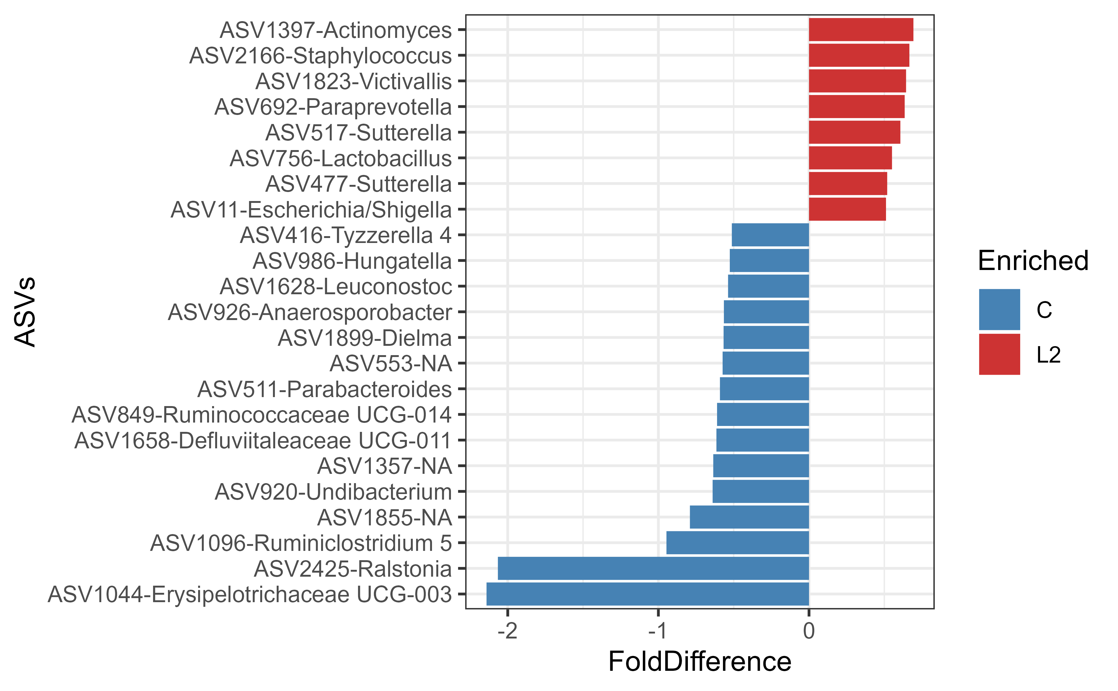
sessionInfo()
#> R version 4.2.1 (2022-06-23 ucrt)
#> Platform: x86_64-w64-mingw32/x64 (64-bit)
#> Running under: Windows 10 x64 (build 19044)
#>
#> Matrix products: default
#>
#> locale:
#> [1] LC_COLLATE=English_United States.utf8
#> [2] LC_CTYPE=English_United States.utf8
#> [3] LC_MONETARY=English_United States.utf8
#> [4] LC_NUMERIC=C
#> [5] LC_TIME=English_United States.utf8
#>
#> attached base packages:
#> [1] stats     graphics  grDevices utils     datasets  methods   base
#>
#> other attached packages:
#> [1] dplyr_1.0.9       biomeUtils_0.020  microbiome_1.18.0 ggplot2_3.3.6
#> [5] phyloseq_1.40.0
#>
#> loaded via a namespace (and not attached):
#>   [1] nlme_3.1-157           bitops_1.0-7           fs_1.5.2
#>   [4] bit64_4.0.5            rprojroot_2.0.3        GenomeInfoDb_1.32.2
#>   [7] tools_4.2.1            bslib_0.4.0            utf8_1.2.2
#>  [10] R6_2.5.1               vegan_2.6-2            DBI_1.1.3
#>  [13] BiocGenerics_0.42.0    mgcv_1.8-40            colorspace_2.0-3
#>  [16] permute_0.9-7          rhdf5filters_1.8.0     ade4_1.7-19
#>  [19] withr_2.5.0            phangorn_2.10.0        tidyselect_1.1.2
#>  [22] bit_4.0.4              compiler_4.2.1         textshaping_0.3.6
#>  [25] cli_3.3.0              Biobase_2.56.0         desc_1.4.2
#>  [28] labeling_0.4.2         sass_0.4.2             scales_1.2.1
#>  [31] quadprog_1.5-8         pkgdown_2.0.6          systemfonts_1.0.4
#>  [34] stringr_1.4.1          digest_0.6.29          rmarkdown_2.16
#>  [37] XVector_0.36.0         pkgconfig_2.0.3        htmltools_0.5.3
#>  [40] highr_0.9              fastmap_1.1.0          rlang_1.0.5
#>  [43] RSQLite_2.2.14         rstudioapi_0.14        farver_2.1.1
#>  [46] jquerylib_0.1.4        generics_0.1.3         jsonlite_1.8.0
#>  [49] RCurl_1.98-1.6         magrittr_2.0.3         GenomeInfoDbData_1.2.8
#>  [52] biomformat_1.24.0      Matrix_1.5-1           Rcpp_1.0.8.3
#>  [55] munsell_0.5.0          S4Vectors_0.34.0       Rhdf5lib_1.18.2
#>  [58] fansi_1.0.3            DECIPHER_2.24.0        ape_5.6-2
#>  [61] lifecycle_1.0.2        stringi_1.7.6          yaml_2.3.5
#>  [64] MASS_7.3-57            zlibbioc_1.42.0        rhdf5_2.40.0
#>  [67] Rtsne_0.16             plyr_1.8.7             blob_1.2.3
#>  [70] grid_4.2.1             parallel_4.2.1         crayon_1.5.1
#>  [73] lattice_0.20-45        Biostrings_2.64.0      splines_4.2.1
#>  [76] multtest_2.52.0        knitr_1.40             pillar_1.8.1
#>  [79] igraph_1.3.1           reshape2_1.4.4         codetools_0.2-18
#>  [82] stats4_4.2.1           fastmatch_1.1-3        picante_1.8.2
#>  [85] glue_1.6.2             evaluate_0.16          data.table_1.14.2
#>  [88] vctrs_0.4.1            foreach_1.5.2          gtable_0.3.1
#>  [91] purrr_0.3.4            tidyr_1.2.0            assertthat_0.2.1
#>  [94] cachem_1.0.6           xfun_0.31              ragg_1.2.2
#>  [97] survival_3.3-1         tibble_3.1.7           iterators_1.0.14
#> [100] memoise_2.0.1          IRanges_2.30.0         cluster_2.1.3
#> [103] ellipsis_0.3.2